预测自行车出行次数
在本教程中,构建一个机器学习应用程序来预测下一个骑行时段从一个车站出发的自行车出行次数。该应用程序包含三个重要步骤:
预测工程
特征工程
机器学习
第一步,使用 Compose 从数据中创建新标签。第二步,使用 Featuretools 为标签生成特征。第三步,使用 EvalML 搜索最佳机器学习管道。完成这些步骤后,你应该了解如何构建机器学习应用程序来解决预测需求等实际问题。
注意:为了运行此示例,你应该安装 Featuretools 1.4.0 或更新版本,以及 EvalML 0.41.0 或更新版本。
[1]:
from demo.chicago_bike import load_sample
from matplotlib.pyplot import subplots
import composeml as cp
import featuretools as ft
import evalml
使用 Divvy(芝加哥的自行车共享服务)提供的数据。在此数据集中,我们有每次自行车出行的记录。
[2]:
df = load_sample()
df.head()
[2]:
| 性别 (gender) | 开始时间 (starttime) | 结束时间 (stoptime) | 出行时长 (tripduration) | 温度 (temperature) | 事件 (events) | 起始车站 ID (from_station_id) | 起始停车容量 (dpcapacity_start) | 结束车站 ID (to_station_id) | 结束停车容量 (dpcapacity_end) | |
|---|---|---|---|---|---|---|---|---|---|---|
| 出行 ID (trip_id) | ||||||||||
| 2331610 | 女性 | 2014-06-29 13:35:00 | 2014-06-29 13:56:00 | 20.750000 | 82.9 | 多云 | 178 | 15.0 | 76 | 39.0 |
| 2347603 | 女性 | 2014-06-30 12:07:00 | 2014-06-30 12:37:00 | 30.150000 | 82.0 | 多云 | 211 | 19.0 | 177 | 15.0 |
| 2345120 | 男性 | 2014-06-30 08:36:00 | 2014-06-30 08:43:00 | 6.516667 | 75.0 | 多云 | 340 | 15.0 | 67 | 15.0 |
| 2347527 | 男性 | 2014-06-30 12:00:00 | 2014-06-30 12:08:00 | 7.250000 | 82.0 | 多云 | 56 | 19.0 | 56 | 19.0 |
| 2344421 | 男性 | 2014-06-30 08:04:00 | 2014-06-30 08:11:00 | 7.316667 | 75.0 | 多云 | 77 | 23.0 | 37 | 19.0 |
预测工程
下一个骑行时段将有多少次从某个车站出发的出行?
你可以更改骑行时段的长度来创建不同的预测问题。例如,在接下来的 13 小时或下一周内将发生多少次自行车出行?这些变化可以通过简单地调整一个参数来完成。这有助于你理解对于做出更好决策至关重要的不同场景。
定义标签函数
定义一个标签函数来计算出行次数。鉴于每个观测值是一次单独的出行,出行次数就是观测值的数量。你的标签函数应该由标签生成器使用来提取训练样本。
[3]:
def trip_count(ds):
    return len(ds)
表示预测问题
通过创建具有以下参数的标签生成器来表示预测问题:
target_dataframe_index作为出行起始车站 ID 的列,因为你想处理来自每个车站的出行。labeling_function作为计算出行次数的函数。time_index作为出行开始时间的列。骑行时段基于此时间索引。window_size作为骑行时段的长度。你可以轻松更改此参数来创建预测问题的变体。
[4]:
lm = cp.LabelMaker(
    target_dataframe_index='from_station_id',
    labeling_function=trip_count,
    time_index='starttime',
    window_size='13h',
)
查找训练样本
使用以下参数运行搜索以获取训练样本:
按开始时间排序的出行数据,因为搜索期望出行数据按时间顺序排序,否则会引发错误。
num_examples_per_instance用于查找每个车站的训练样本数量。在这种情况下,搜索返回所有现有样本。minimum_data作为第一个骑行时段的开始时间。这也是构建特征的第一个截止时间。
[5]:
lt = lm.search(
    df.sort_values('starttime'),
    num_examples_per_instance=-1,
    minimum_data='2014-06-30 08:00',
    verbose=False,
)

lt.head()
[5]:
| 起始车站 ID (from_station_id) | 时间 (time) | 出行次数 (trip_count) | |
|---|---|---|---|
| 0 | 5 | 2014-06-30 08:00:00 | 3 |
| 1 | 15 | 2014-06-30 08:00:00 | 1 |
| 2 | 16 | 2014-06-30 08:00:00 | 1 |
| 3 | 17 | 2014-06-30 08:00:00 | 2 |
| 4 | 19 | 2014-06-30 08:00:00 | 2 |
搜索的输出是一个包含三列的标签时间表:
与出行相关的车站 ID。每个车站可以生成多个训练样本。
骑行时段的开始时间。这也是构建特征的截止时间。仅限在此之前存在的数据可用于预测。
骑行时段窗口内的出行次数。这由我们的标签函数计算。
作为有用的参考,你可以打印出用于生成这些标签的搜索设置。
[6]:
lt.describe()
Label Distribution
------------------
count    212.000000
mean       2.669811
std        2.367720
min        1.000000
25%        1.000000
50%        2.000000
75%        3.000000
max       13.000000


Settings
--------
gap                                      None
maximum_data                             None
minimum_data                 2014-06-30 08:00
num_examples_per_instance                  -1
target_column                      trip_count
target_dataframe_index        from_station_id
target_type                        continuous
window_size                               13h


Transforms
----------
No transforms applied
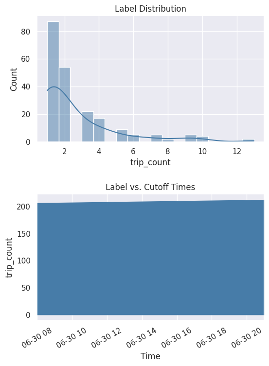
你还可以通过绘制分布和随时间的累积计数来更好地查看标签。
[7]:
%matplotlib inline
fig, ax = subplots(nrows=2, ncols=1, figsize=(6, 8))
lt.plot.distribution(ax=ax[0])
lt.plot.count_by_time(ax=ax[1])
fig.tight_layout(pad=2)
特征工程
在上一步中,你生成了标签。下一步是生成特征。
表示数据
首先使用 EntitySet 来表示数据。这样,你可以根据数据集的关系结构生成特征。你当前有一个单一的出行表,其中一个车站可以有多次出行。这种一对多关系可以通过规范化车站数据框来表示。同样的操作也可以应用于天气与出行等其他一对多关系。因为你想根据出行起始的车站进行预测,你应该使用这个车站数据框作为生成特征的目标。此外,你应该使用出行结束时间作为生成特征的时间索引,因为直到出行完成,有关出行的数据可能才可用。
[8]:
es = ft.EntitySet('chicago_bike')

es.add_dataframe(
    dataframe=df.reset_index(),
    dataframe_name='trips',
    time_index='stoptime',
    index='trip_id',
)

es.normalize_dataframe(
    base_dataframe_name='trips',
    new_dataframe_name='from_station_id',
    index='from_station_id',
    make_time_index=False,
)

es.normalize_dataframe(
    base_dataframe_name='trips',
    new_dataframe_name='weather',
    index='events',
    make_time_index=False,
)

es.normalize_dataframe(
    base_dataframe_name='trips',
    new_dataframe_name='gender',
    index='gender',
    make_time_index=False,
)

es.add_interesting_values(dataframe_name='trips',
                          values={'gender': ['Male', 'Female'],
                                  'events': ['tstorms']})
es.plot()
[8]:

计算特征
使用称为深度特征合成 (Deep Feature Synthesis, DFS) 的方法生成特征。该方法通过在实体集中的关系上堆叠和应用称为“基本操作”(primitives) 的数学运算来自动构建特征。实体集的结构化程度越高,DFS 就能更好地利用关系来生成更好的特征。使用以下参数运行 DFS:
entityset作为我们之前构建的实体集。target_dataframe_name作为出行起始的车站数据框。cutoff_time作为我们之前生成的标签时间。标签值会附加到特征矩阵。
[9]:
fm, fd = ft.dfs(
    entityset=es,
    target_dataframe_name='from_station_id',
    trans_primitives=['hour', 'week', 'is_weekend'],
    cutoff_time=lt,
    cutoff_time_in_index=True,
    include_cutoff_time=False,
    verbose=False,
)

fm.head()
[9]:
| COUNT(trips) | MAX(trips.dpcapacity_end) | MAX(trips.dpcapacity_start) | MAX(trips.temperature) | MAX(trips.to_station_id) | MAX(trips.tripduration) | MEAN(trips.dpcapacity_end) | MEAN(trips.dpcapacity_start) | MEAN(trips.temperature) | MEAN(trips.to_station_id) | ... | MODE(trips.HOUR(stoptime)) | MODE(trips.WEEK(starttime)) | MODE(trips.WEEK(stoptime)) | NUM_UNIQUE(trips.HOUR(starttime)) | NUM_UNIQUE(trips.HOUR(stoptime)) | NUM_UNIQUE(trips.WEEK(starttime)) | NUM_UNIQUE(trips.WEEK(stoptime)) | PERCENT_TRUE(trips.IS_WEEKEND(starttime)) | PERCENT_TRUE(trips.IS_WEEKEND(stoptime)) | 出行次数 (trip_count) | ||
|---|---|---|---|---|---|---|---|---|---|---|---|---|---|---|---|---|---|---|---|---|---|---|
| 起始车站 ID (from_station_id) | 时间 (time) | |||||||||||||||||||||
| 5 | 2014-06-30 08:00:00 | 1 | 39.0 | 19.0 | 84.0 | 76.0 | 9.233333 | 39.000000 | 19.0 | 84.000000 | 76.000000 | ... | 14 | 26 | 26 | 1 | 1 | 1 | 1 | 1.000000 | 1.000000 | 3 |
| 15 | 2014-06-30 08:00:00 | 3 | 19.0 | 15.0 | 84.2 | 280.0 | 14.166667 | 16.333333 | 15.0 | 76.733333 | 137.333333 | ... | 7 | 27 | 27 | 3 | 2 | 2 | 2 | 0.333333 | 0.333333 | 1 |
| 16 | 2014-06-30 08:00:00 | 2 | 15.0 | 11.0 | 84.9 | 340.0 | 25.083333 | 13.000000 | 11.0 | 84.900000 | 324.500000 | ... | 17 | 26 | 26 | 1 | 2 | 1 | 1 | 1.000000 | 1.000000 | 1 |
| 17 | 2014-06-30 08:00:00 | 1 | 15.0 | 15.0 | 84.9 | 183.0 | 4.650000 | 15.000000 | 15.0 | 84.900000 | 183.000000 | ... | 17 | 26 | 26 | 1 | 1 | 1 | 1 | 1.000000 | 1.000000 | 2 |
| 19 | 2014-06-30 08:00:00 | 0 | NaN | NaN | NaN | NaN | NaN | NaN | NaN | NaN | NaN | ... | NaN | NaN | NaN | <NA> | <NA> | <NA> | <NA> | 0.000000 | 0.000000 | 2 |
5 行 x 49 列
DFS 的输出有两个:一个特征矩阵和特征定义。特征矩阵是一个表格,包含基于截止时间的特征值和相应的标签。特征定义是列表中的特征,可以存储起来并在以后重用,以便在未来数据上计算同一组特征。
机器学习
在前面的步骤中,你生成了标签和特征。最后一步是构建机器学习管道。
分割数据
首先从特征矩阵中提取标签,并将数据分割成训练集和保留集。
[10]:
fm.reset_index(drop=True, inplace=True)
y = fm.ww.pop('trip_count')

splits = evalml.preprocessing.split_data(
    X=fm,
    y=y,
    test_size=0.1,
    random_seed=0,
    problem_type='regression',
)

X_train, X_holdout, y_train, y_holdout = splits
查找最佳模型
在训练集上运行搜索以查找最佳机器学习模型。在搜索过程中,会评估来自多个不同管道的预测。
[11]:
automl = evalml.AutoMLSearch(
    X_train=X_train,
    y_train=y_train,
    problem_type='regression',
    objective='r2',
    random_seed=3,
    allowed_model_families=['extra_trees', 'random_forest'],
    max_iterations=3,
)

automl.search()
[11]:
{1: {'Elastic Net Regressor w/ Replace Nullable Types Transformer + Imputer + One Hot Encoder + Standard Scaler': '00:02',
  'Random Forest Regressor w/ Replace Nullable Types Transformer + Imputer + One Hot Encoder': '00:02',
  'Total time of batch': '00:04'}}
搜索完成后,你可以打印出有关最佳管道的信息,例如每个组件中的参数。
[12]:
automl.best_pipeline.describe()
automl.best_pipeline.graph()
*********************************************************************************************
* Random Forest Regressor w/ Replace Nullable Types Transformer + Imputer + One Hot Encoder *
*********************************************************************************************

Problem Type: regression
Model Family: Random Forest
Number of features: 84

Pipeline Steps
==============
1. Replace Nullable Types Transformer
2. Imputer
         * categorical_impute_strategy : most_frequent
         * numeric_impute_strategy : mean
         * boolean_impute_strategy : most_frequent
         * categorical_fill_value : None
         * numeric_fill_value : None
         * boolean_fill_value : None
3. One Hot Encoder
         * top_n : 10
         * features_to_encode : None
         * categories : None
         * drop : if_binary
         * handle_unknown : ignore
         * handle_missing : error
4. Random Forest Regressor
         * n_estimators : 100
         * max_depth : 6
         * n_jobs : -1
[12]:

让我们通过评估在保留集上的预测来对模型性能进行评分。
[13]:
best_pipeline = automl.best_pipeline.fit(X_train, y_train)

score = best_pipeline.score(
    X=X_holdout,
    y=y_holdout,
    objectives=['r2'],
)

dict(score)
[13]:
{'R2': 0.15991282341144752}
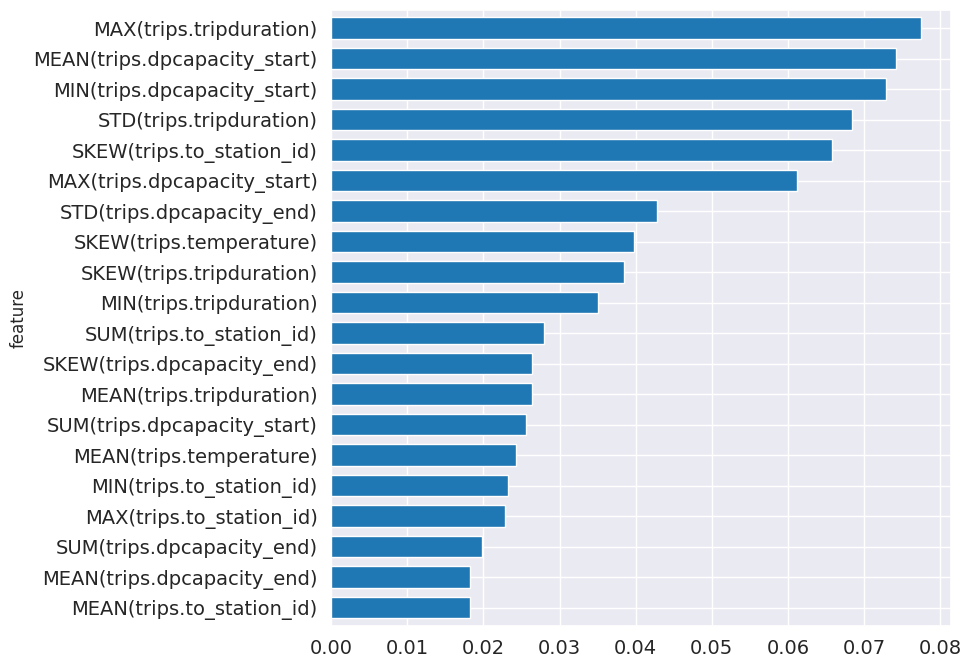
从管道中,你可以看到哪些特征对预测最重要。
[14]:
feature_importance = best_pipeline.feature_importance
feature_importance = feature_importance.set_index('feature')['importance']
top_k = feature_importance.abs().sort_values().tail(20).index
feature_importance[top_k].plot.barh(figsize=(8, 8), fontsize=14, width=.7);
进行预测
现在你可以使用训练好的模型进行预测了。首先使用特征定义计算同一组特征。然后使用基于数据集中最新可用信息的截止时间。
[15]:
fm = ft.calculate_feature_matrix(
    features=fd,
    entityset=es,
    cutoff_time=ft.pd.Timestamp('2014-07-02 08:00:00'),
    cutoff_time_in_index=True,
    verbose=False,
)

fm.head()
[15]:
| COUNT(trips) | MAX(trips.dpcapacity_end) | MAX(trips.dpcapacity_start) | MAX(trips.temperature) | MAX(trips.to_station_id) | MAX(trips.tripduration) | MEAN(trips.dpcapacity_end) | MEAN(trips.dpcapacity_start) | MEAN(trips.temperature) | MEAN(trips.to_station_id) | ... | MODE(trips.HOUR(starttime)) | MODE(trips.HOUR(stoptime)) | MODE(trips.WEEK(starttime)) | MODE(trips.WEEK(stoptime)) | NUM_UNIQUE(trips.HOUR(starttime)) | NUM_UNIQUE(trips.HOUR(stoptime)) | NUM_UNIQUE(trips.WEEK(starttime)) | NUM_UNIQUE(trips.WEEK(stoptime)) | PERCENT_TRUE(trips.IS_WEEKEND(starttime)) | PERCENT_TRUE(trips.IS_WEEKEND(stoptime)) | ||
|---|---|---|---|---|---|---|---|---|---|---|---|---|---|---|---|---|---|---|---|---|---|---|
| 起始车站 ID (from_station_id) | 时间 (time) | |||||||||||||||||||||
| 186 | 2014-07-02 08:00:00 | 1 | 19.0 | 15.0 | 82.9 | 56.0 | 6.483333 | 19.000000 | 15.0 | 82.900000 | 56.000000 | ... | 13 | 13 | 26 | 26 | 1 | 1 | 1 | 1 | 1.00000 | 1.00000 |
| 181 | 2014-07-02 08:00:00 | 8 | 27.0 | 31.0 | 84.9 | 233.0 | 18.350000 | 20.500000 | 31.0 | 83.212500 | 140.750000 | ... | 16 | 16 | 27 | 27 | 5 | 5 | 2 | 2 | 0.37500 | 0.37500 |
| 177 | 2014-07-02 08:00:00 | 23 | 31.0 | 15.0 | 84.9 | 334.0 | 50.233333 | 17.434783 | 15.0 | 83.334783 | 219.565217 | ... | 16 | 18 | 26 | 26 | 8 | 8 | 2 | 2 | 0.73913 | 0.73913 |
| 13 | 2014-07-02 08:00:00 | 3 | 19.0 | 19.0 | 82.9 | 165.0 | 13.916667 | 17.666667 | 19.0 | 82.600000 | 112.666667 | ... | 13 | 13 | 26 | 26 | 2 | 2 | 1 | 1 | 1.00000 | 1.00000 |
| 153 | 2014-07-02 08:00:00 | 2 | 23.0 | 19.0 | 82.9 | 324.0 | 13.850000 | 19.000000 | 19.0 | 77.950000 | 219.500000 | ... | 6 | 6 | 26 | 26 | 2 | 2 | 2 | 2 | 0.50000 | 0.50000 |
5 行 x 48 列
预测下一个 13 小时内从一个车站出发的出行次数。
[16]:
y_pred = best_pipeline.predict(fm)
y_pred = y_pred.values.round()

prediction = fm[[]]
prediction['trip_count (estimate)'] = y_pred
prediction.head()
[16]:
| 出行次数(估计) | ||
|---|---|---|
| 起始车站 ID (from_station_id) | 时间 (time) | |
| 186 | 2014-07-02 08:00:00 | 1.0 |
| 181 | 2014-07-02 08:00:00 | 4.0 |
| 177 | 2014-07-02 08:00:00 | 5.0 |
| 13 | 2014-07-02 08:00:00 | 4.0 |
| 153 | 2014-07-02 08:00:00 | 3.0 |
下一步
你已完成本教程。你可以回顾每个步骤,使用不同的参数探索和微调模型,直到它准备好投入生产。有关如何使用 Featuretools 生成的特征的更多信息,请查看 Featuretools 文档。有关如何使用 EvalML 生成的模型的更多信息,请查看 EvalML 文档。