预测涡轮风扇性能退化¶

在本教程中，我们将构建一个机器学习应用程序来预测涡轮风扇发动机的性能退化。此应用程序分为三个重要步骤

预测工程
特征工程
机器学习

第一步，使用 Compose 从数据中创建新标签。第二步，使用 Featuretools 为这些标签生成特征。第三步，使用 EvalML 搜索最佳机器学习管道。完成这些步骤后，您应该了解如何为预测需求等实际问题构建机器学习应用程序。

注意：为了运行此示例，您应该安装 Featuretools 1.4.0 或更高版本以及 EvalML 0.41.0 或更高版本。

[1]:

from demo.turbofan_degredation import load_sample
from matplotlib.pyplot import subplots
import composeml as cp
import featuretools as ft
import evalml

使用由 NASA 提供的数据集，该数据集模拟了涡轮风扇发动机的性能退化。数据集中包含随时间受到监控的发动机数据。每台发动机都在多个周期内记录了操作设置和传感器测量值。剩余使用寿命 (RUL) 是发动机在需要维护之前剩余的循环次数。这个数据集的特别之处在于发动机一直运行到失效，从而为我们提供了每台发动机在每个时间点的精确 RUL 信息。您在本教程中构建的模型将预测 RUL。

[2]:

df = load_sample()
df.head()

[2]:

	engine_no	time_in_cycles	operational_setting_1	operational_setting_2	operational_setting_3	sensor_measurement_1	sensor_measurement_2	sensor_measurement_3	sensor_measurement_4	sensor_measurement_5	...	sensor_measurement_13	sensor_measurement_14	sensor_measurement_15	sensor_measurement_16	sensor_measurement_17	sensor_measurement_18	sensor_measurement_19	sensor_measurement_20	sensor_measurement_21	time
id
270	1	271	0.0010	0.0018	100.0	518.67	643.01	1591.11	1395.60	14.62	...	2388.12	8157.56	8.3141	0.03	393	2388	100.0	39.26	23.5280	2000-01-02 21:00:00
401	2	81	0.0004	0.0000	100.0	518.67	642.88	1581.74	1398.46	14.62	...	2387.98	8134.70	8.4092	0.03	392	2388	100.0	39.08	23.3215	2000-01-03 18:50:00
810	3	191	41.9983	0.8400	100.0	445.00	549.13	1352.21	1122.64	3.91	...	2388.18	8098.80	9.2919	0.02	330	2212	100.0	10.64	6.4525	2000-01-06 15:00:00
66	1	67	35.0054	0.8400	100.0	449.44	555.43	1351.45	1109.90	5.48	...	2387.89	8062.45	9.3215	0.02	333	2223	100.0	14.90	9.0315	2000-01-01 11:00:00
328	2	8	0.0023	0.0019	100.0	518.67	642.23	1576.51	1391.71	14.62	...	2388.07	8135.66	8.3894	0.03	392	2388	100.0	38.95	23.4243	2000-01-03 06:40:00

5 行 × 27 列

预测工程¶

涡轮风扇发动机的 RUL 在哪个范围内？

在这个预测问题中，您希望将 RUL 数据分组到不同的范围，然后预测 RUL 所在的范围。您可以改变范围来创建不同的预测问题。例如，范围可以是手动定义（0 - 150、150 - 300 等），或者基于历史观测数据的四分位数。对 RUL 进行分箱，有助于您探索对于做出更好决策至关重要的不同场景。

定义标签函数¶

我们首先定义一个计算发动机 RUL 的标签函数。考虑到发动机一直运行到失效，RUL 就是剩余的观测次数。我们的标签函数将被标签生成器用于提取训练样本。

[3]:

def rul(ds):
    return len(ds) - 1

表示预测问题¶

通过创建具有以下参数的标签生成器来表示预测问题

将 target_dataframe_index 作为发动机 ID 的列，因为您希望处理每台发动机的记录。
将 labeling_function 作为您之前定义的函数。
将 time_index 作为事件时间的列。

[4]:

lm = cp.LabelMaker(
    target_dataframe_index='engine_no',
    labeling_function=rul,
    time_index='time',
)

寻找训练样本¶

使用以下参数运行搜索以获取训练样本

按事件时间排序的记录，因为搜索期望记录按时间顺序排列。否则，会发生错误。
将 num_examples_per_instance 作为为每台发动机找到的训练样本数量。
将 minimum_data 作为用于为第一个训练样本生成特征的数据量。
将 gap 作为样本之间跳过的行数。这样做是为了覆盖发动机在不同时间点的情况。

您可以轻松调整这些参数并运行更多训练样本搜索，以应对模型需求的变化。

[5]:

lt = lm.search(
    df.sort_values('time'),
    num_examples_per_instance=20,
    minimum_data=5,
    gap=20,
    verbose=False,
)

lt.head()

[5]:

	engine_no	time	rul
0	1	2000-01-01 02:10:00	153
1	1	2000-01-01 10:20:00	133
2	1	2000-01-01 15:30:00	113
3	1	2000-01-02 00:20:00	93
4	1	2000-01-02 06:00:00	73

搜索的输出是一个标签时间表，包含三列

与记录相关的发动机 ID。每台发动机可以生成许多训练样本。
发动机的事件时间。这也称为构建特征的截止时间。只有在此时间之前存在的数据才有效，可用于预测。
RUL 的值。这是由标签函数计算得出的。

此时，您只有 RUL 的连续值。作为有用的参考，您可以打印出用于生成这些标签的搜索设置。

[6]:

lt.describe()

Label Distribution
------------------
count     22.000000
mean      75.045455
std       43.795496
min        6.000000
25%       37.750000
50%       74.000000
75%      111.250000
max      153.000000


Settings
--------
gap                                  20
maximum_data                       None
minimum_data                          5
num_examples_per_instance            20
target_column                       rul
target_dataframe_index        engine_no
target_type                  continuous
window_size                        None


Transforms
----------
No transforms applied

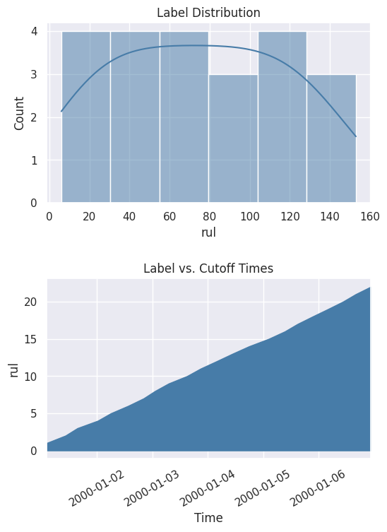
您还可以通过绘制分布图和累积计数图来更好地查看这些值。

[7]:

%matplotlib inline
fig, ax = subplots(nrows=2, ncols=1, figsize=(6, 8))
lt.plot.distribution(ax=ax[0])
lt.plot.count_by_time(ax=ax[1])
fig.tight_layout(pad=2)

../_images/examples_predict_turbofan_degredation_13_0.png

有了连续值，您无需再次运行搜索即可探索不同的范围。在这种情况下，使用四分位数将值分箱到不同的范围。

[8]:

lt = lt.bin(4, quantiles=True, precision=0)

当您再次打印出设置时，您现在可以看到标签的描述已更新，并反映了最新的更改。

[9]:

lt.describe()

Label Distribution
------------------
(5.0, 38.0]        6
(38.0, 74.0]       5
(74.0, 111.0]      5
(111.0, 153.0]     6
Total:            22


Settings
--------
gap                                 20
maximum_data                      None
minimum_data                         5
num_examples_per_instance           20
target_column                      rul
target_dataframe_index       engine_no
target_type                   discrete
window_size                       None


Transforms
----------
1. bin
  - bins:            4
  - labels:       None
  - precision:       0
  - quantiles:    True
  - right:        True

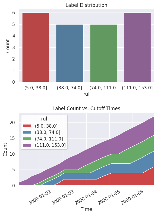
查看新的标签分布和随时间变化的累积计数。

[10]:

fig, ax = subplots(nrows=2, ncols=1, figsize=(6, 8))
lt.plot.distribution(ax=ax[0])
lt.plot.count_by_time(ax=ax[1])
fig.tight_layout(pad=2)

../_images/examples_predict_turbofan_degredation_19_0.png

特征工程¶

在上一步中，您生成了标签。下一步是生成特征。

表示数据¶

我们首先使用 EntitySet 来表示数据。这样，您可以基于数据集的关系结构生成特征。您当前拥有一张记录表，其中一台发动机可以有多条记录。这种一对多关系可以通过规范化发动机数据框来表示。其他一对多关系也可以同样处理。因为您希望基于发动机进行预测，所以应该使用此发动机数据框作为生成特征的目标。

[11]:

es = ft.EntitySet('observations')

es.add_dataframe(
    dataframe=df.reset_index(),
    dataframe_name='records',
    index='id',
    time_index='time',
)

es.normalize_dataframe(
    base_dataframe_name='records',
    new_dataframe_name='engines',
    index='engine_no',
)

es.normalize_dataframe(
    base_dataframe_name='records',
    new_dataframe_name='cycles',
    index='time_in_cycles',
)

es.plot()

[11]:

../_images/examples_predict_turbofan_degredation_21_0.svg

计算特征¶

现在，您可以使用称为深度特征合成 (Deep Feature Synthesis, DFS) 的方法生成特征。该方法通过在实体集中的关系上堆叠和应用称为基元的数学运算来自动构建特征。实体集结构越好，DFS 就能越好地利用这些关系来生成更好的特征。使用以下参数运行 DFS

将 entityset 作为我们之前构建的实体集。
将 target_dataframe_name 作为发动机数据框。
将 cutoff_time 作为我们之前生成的标签时间。标签值将附加到特征矩阵中。

[12]:

fm, fd = ft.dfs(
    entityset=es,
    target_dataframe_name='engines',
    agg_primitives=['sum'],
    trans_primitives=[],
    cutoff_time=lt,
    cutoff_time_in_index=True,
    include_cutoff_time=False,
    verbose=False,
)

fm.head()

[12]:

		SUM(records.operational_setting_1)	SUM(records.operational_setting_2)	SUM(records.operational_setting_3)	SUM(records.sensor_measurement_1)	SUM(records.sensor_measurement_10)	SUM(records.sensor_measurement_11)	SUM(records.sensor_measurement_12)	SUM(records.sensor_measurement_13)	SUM(records.sensor_measurement_14)	SUM(records.sensor_measurement_15)	...	SUM(records.sensor_measurement_20)	SUM(records.sensor_measurement_21)	SUM(records.sensor_measurement_3)	SUM(records.sensor_measurement_4)	SUM(records.sensor_measurement_5)	SUM(records.sensor_measurement_6)	SUM(records.sensor_measurement_7)	SUM(records.sensor_measurement_8)	SUM(records.sensor_measurement_9)	rul
engine_no	time
1	2000-01-01 02:10:00	144.0091	3.1408	460.0	2320.65	5.29	207.99	1125.75	11579.85	40197.21	47.2120	...	88.81	53.7315	6888.78	5769.91	34.97	49.96	1196.94	10949.70	42003.06	(111.0, 153.0]
	2000-01-01 10:20:00	696.0567	16.5674	2340.0	11679.31	26.46	1048.19	5771.01	58258.12	201039.56	235.5492	...	457.84	275.0327	34711.17	29110.65	178.43	255.68	6133.60	55278.36	210997.96	(111.0, 153.0]
	2000-01-01 15:30:00	1074.1074	26.1125	4340.0	21363.69	49.45	1932.52	12306.22	106015.78	362843.58	414.1002	...	961.65	577.5433	64026.68	54108.93	366.96	532.23	13073.84	101404.29	384766.02	(111.0, 153.0]
	2000-01-02 00:20:00	1507.1531	36.1607	6300.0	30844.92	72.28	2799.74	18039.10	153414.42	524573.72	594.5083	...	1409.19	845.9532	92685.14	78469.12	534.32	776.40	19160.56	146707.66	556304.58	(74.0, 111.0]
	2000-01-02 06:00:00	1916.1945	46.6147	8180.0	40426.89	94.48	3658.46	23971.12	200093.76	685705.98	779.0373	...	1872.64	1124.1869	121291.99	102704.45	712.65	1033.81	25466.22	191571.92	727679.61	(38.0, 74.0]

5 行 × 25 列

DFS 有两个输出：特征矩阵和特征定义。特征矩阵是一个表格，包含基于截止时间的特征值和相应的标签。特征定义是存储在列表中的特征，以后可以在未来的数据上重用以计算相同的特征集。

机器学习¶

在前面的步骤中，您生成了标签和特征。最后一步是构建机器学习管道。

拆分数据¶

首先从特征矩阵中提取标签，并将数据拆分为训练集和保留集。

[13]:

fm.reset_index(drop=True, inplace=True)
y = fm.ww.pop('rul').cat.codes

splits = evalml.preprocessing.split_data(
    X=fm,
    y=y,
    test_size=0.2,
    random_seed=2,
    problem_type='multiclass',
)

X_train, X_holdout, y_train, y_holdout = splits

寻找最佳模型¶

在训练集上运行搜索以找到最佳机器学习模型。在搜索过程中，会评估来自不同管道的预测结果以找到最佳管道。

[14]:

automl = evalml.AutoMLSearch(
    X_train=X_train,
    y_train=y_train,
    problem_type='multiclass',
    objective='f1 macro',
    random_seed=0,
    allowed_model_families=['catboost', 'random_forest'],
    max_iterations=3,
)

automl.search()

[14]:

{1: {'Logistic Regression Classifier w/ Label Encoder + Replace Nullable Types Transformer + Imputer + Standard Scaler': '00:02',
  'Random Forest Classifier w/ Label Encoder + Replace Nullable Types Transformer + Imputer': '00:01',
  'Total time of batch': '00:04'}}

搜索完成后，您可以打印出找到的最佳管道的信息，例如每个组件中的参数。

[15]:

automl.best_pipeline.describe()
automl.best_pipeline.graph()

********************************************************************************************************************
* Logistic Regression Classifier w/ Label Encoder + Replace Nullable Types Transformer + Imputer + Standard Scaler *
********************************************************************************************************************

Problem Type: multiclass
Model Family: Linear
Number of features: 24

Pipeline Steps
==============
1. Label Encoder
         * positive_label : None
2. Replace Nullable Types Transformer
3. Imputer
         * categorical_impute_strategy : most_frequent
         * numeric_impute_strategy : mean
         * boolean_impute_strategy : most_frequent
         * categorical_fill_value : None
         * numeric_fill_value : None
         * boolean_fill_value : None
4. Standard Scaler
5. Logistic Regression Classifier
         * penalty : l2
         * C : 1.0
         * n_jobs : -1
         * multi_class : auto
         * solver : lbfgs

[15]:

../_images/examples_predict_turbofan_degredation_29_1.svg

通过在保留集上评估预测结果来评估模型性能。

[16]:

best_pipeline = automl.best_pipeline.fit(X_train, y_train)

score = best_pipeline.score(
    X=X_holdout,
    y=y_holdout,
    objectives=['f1 macro'],
)

dict(score)

[16]:

{'F1 Macro': 0.7}

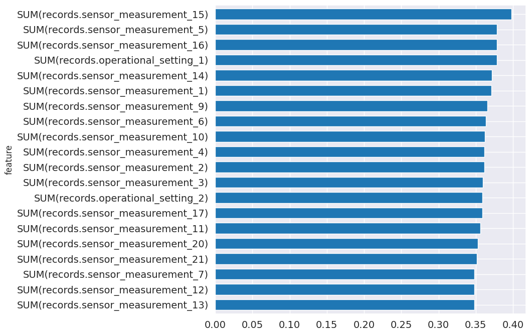
从管道中，您可以看到哪些特征对于预测最重要。

[17]:

feature_importance = best_pipeline.feature_importance
feature_importance = feature_importance.set_index('feature')['importance']
top_k = feature_importance.abs().sort_values().tail(20).index
feature_importance[top_k].plot.barh(figsize=(8, 8), fontsize=14, width=.7);

../_images/examples_predict_turbofan_degredation_33_0.png

进行预测¶

您已准备好使用训练好的模型进行预测。首先使用特征定义计算相同的特征集。使用基于数据集中可用最新信息的截止时间。

[18]:

fm = ft.calculate_feature_matrix(
    features=fd,
    entityset=es,
    cutoff_time=ft.pd.Timestamp('2001-01-08'),
    cutoff_time_in_index=True,
    verbose=False,
)

fm.head()

[18]:

		SUM(records.operational_setting_1)	SUM(records.operational_setting_2)	SUM(records.operational_setting_3)	SUM(records.sensor_measurement_1)	SUM(records.sensor_measurement_10)	SUM(records.sensor_measurement_11)	SUM(records.sensor_measurement_12)	SUM(records.sensor_measurement_13)	SUM(records.sensor_measurement_14)	SUM(records.sensor_measurement_15)	...	SUM(records.sensor_measurement_2)	SUM(records.sensor_measurement_20)	SUM(records.sensor_measurement_21)	SUM(records.sensor_measurement_3)	SUM(records.sensor_measurement_4)	SUM(records.sensor_measurement_5)	SUM(records.sensor_measurement_6)	SUM(records.sensor_measurement_7)	SUM(records.sensor_measurement_8)	SUM(records.sensor_measurement_9)
engine_no	time
1	2001-01-08	3704.4218	88.2459	15140.0	75343.52	176.13	6829.64	43725.78	372863.62	1283533.42	1459.5372	...	92440.87	3417.83	2050.7627	225986.66	191497.63	1302.86	1884.32	46451.89	356328.97	1358639.49
2	2001-01-08	3171.3342	77.7058	13100.0	67022.44	154.92	6045.93	38813.14	327720.14	1135827.75	1317.3793	...	82000.00	3037.99	1821.3241	200451.56	170232.49	1177.62	1696.59	41242.35	313731.51	1202449.71
3	2001-01-08	3158.3517	73.5442	12120.0	62285.84	144.47	5596.92	34594.98	305518.88	1064083.44	1229.1709	...	76036.38	2716.73	1630.8386	185464.99	157035.05	1052.49	1509.15	36748.57	291385.49	1121106.20

3 行 × 24 列

现在预测 RUL 属于四个范围中的哪一个。

[19]:

y_pred = best_pipeline.predict(fm)
y_pred = y_pred.values

prediction = fm[[]]
prediction['rul (estimate)'] = y_pred
prediction.head()

[19]:

		rul (估计值)
engine_no	time
1	2001-01-08	0
2	2001-01-08	0
3	2001-01-08	0

后续步骤¶

您已完成本教程。您可以重新访问每个步骤，使用不同的参数探索和微调模型，直到其准备好投入生产。有关如何使用 Featuretools 生成的特征的更多信息，请查阅 Featuretools 文档。有关如何使用 EvalML 生成的模型的更多信息，请查阅 EvalML 文档。

预测下次购买

用户指南